Jun 29 2020 Antenna for 4G Modem

Simulation accuracy

First, I want to make sure that openEMS (the modeling system I plan to use) is calculating correctly. Let's take the antenna impedance data from the book 1.

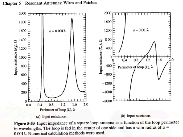
I am interested in the graph on the right, namely the fact that with the perimeter of one square equal to , the reactance .

Let's draw only the top square of the antenna, the feed gap is on the left:

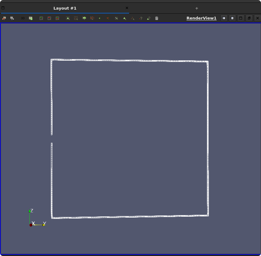
The antenna is a square wire with a side of , effective radius, the length of the full side of the square is , the feed gap is equal to . Thus, the perimeter of the antenna is .

After simulation EndCriteria = 1.e-6, OverSampling = 10 I get the resonant frequency :

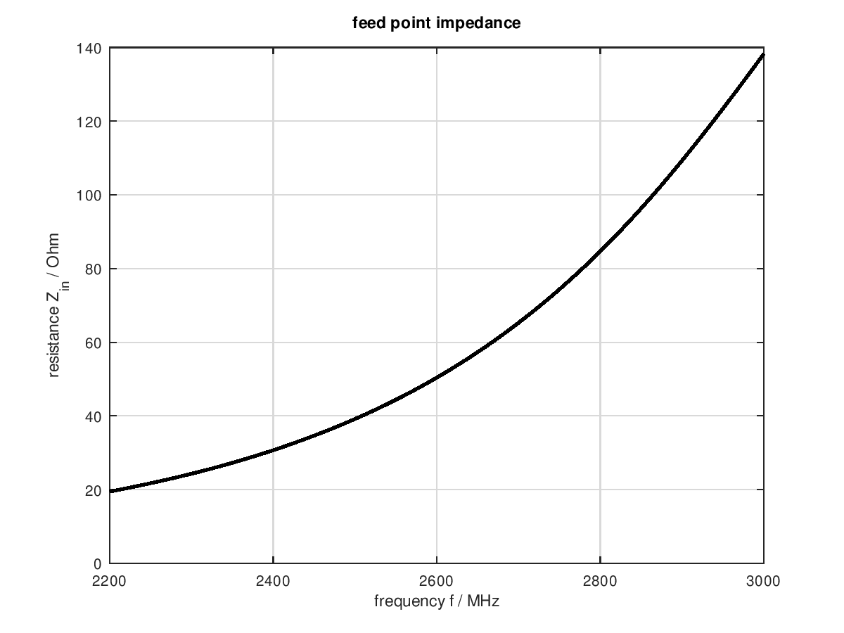
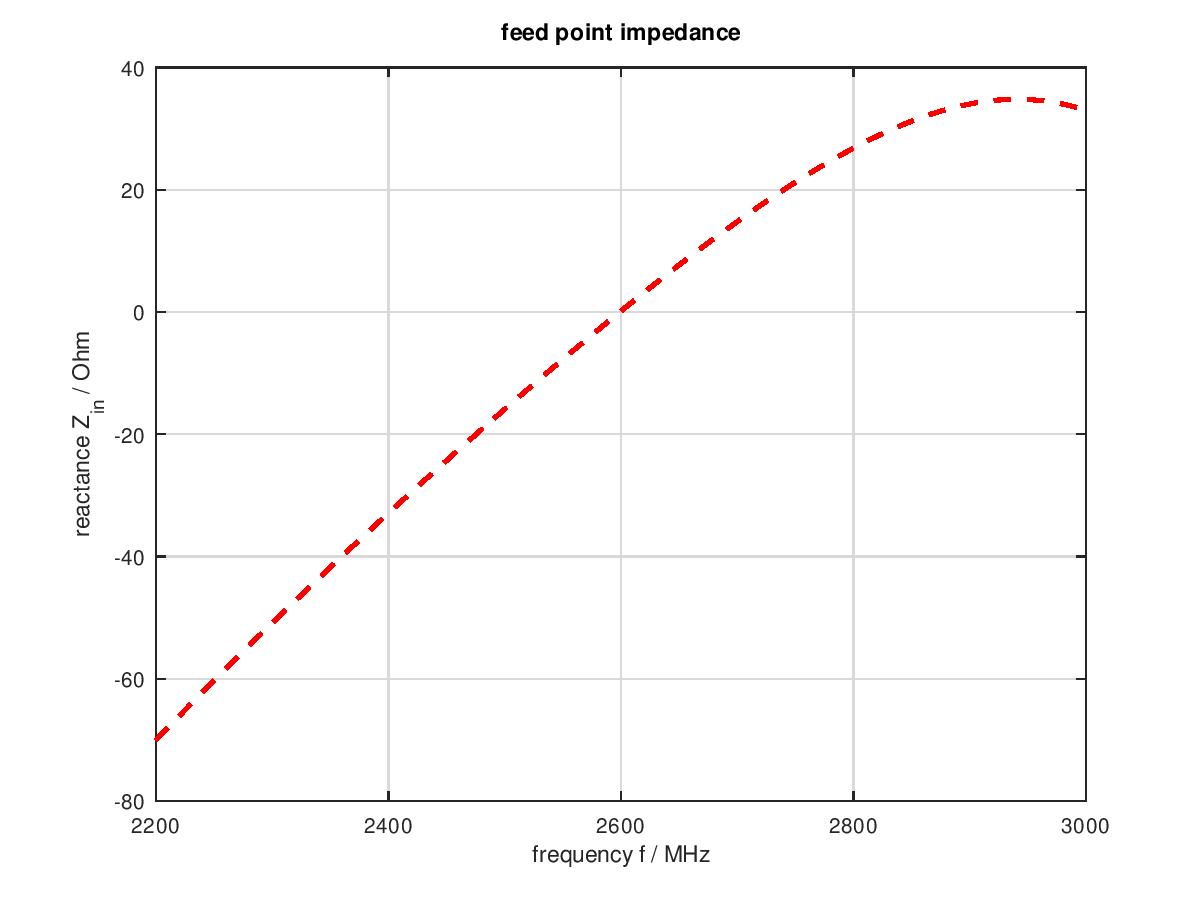
directivity: Dmax = 3.0867 dBi
Minimum SWR frequency:
 2840000000
Resonant frequency (jX=0):
 2865000000
Impedance at minimum SWR:
 129.502 -  13.569i
Impedance at resonant frequency:
 133.07147 -   0.41565i
Minimum SWR:
 2.6234

From the frequency I find the wavelength: and the theoretical perimeter: .

Hence the discrepancy between theory and simulation: . The source code of the simulation can be downloaded here.

Given the artisanal nature of production, this accuracy suits me:)

Antenna geometry

In theory, an antenna is two squares connected by "vertices", where the connection point is the feed point of the antenna. But I will be dealing with a real copper wire (there is a height and thickness), which bends with a certain radius, as well as with a real soldering iron, so that the geometric model will look like this:

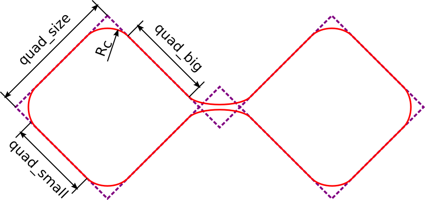
The dotted lines are auxiliary geometry, the red curve is the center of the wire from which the antenna is made, the radii of all arcs are equal to (here means the center).

At this point, I will need the characteristics of my copper wire. It just so happened that I had a lot of rectangular copper wire at hand, so I will be guided by this type of wire.

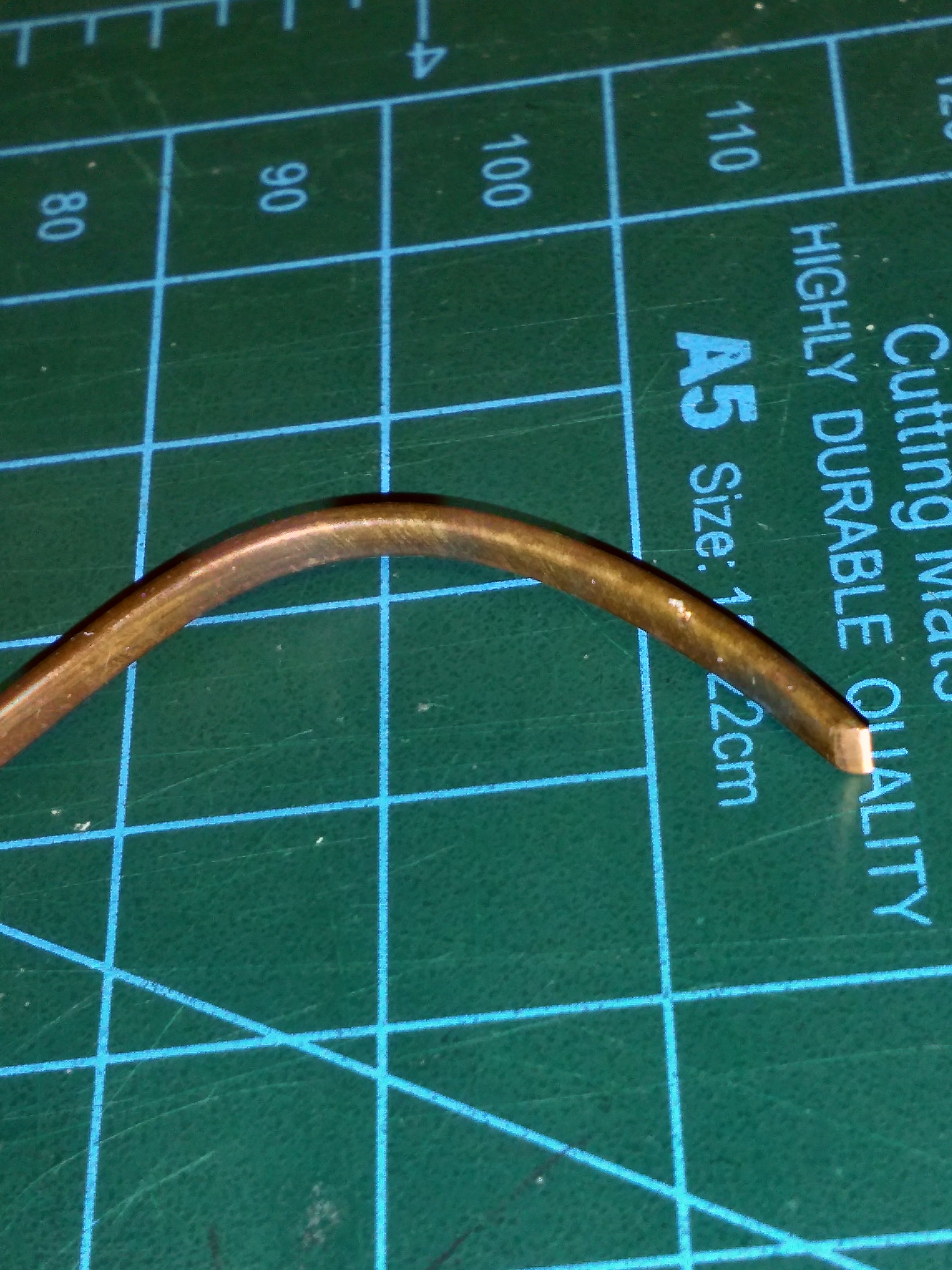
The rectangular cross-section of the wire is described by the width and the height , , hence it is clear how the wire will bend --- I can ignore in the geometric model, but will play an important role in describing the feed gap.

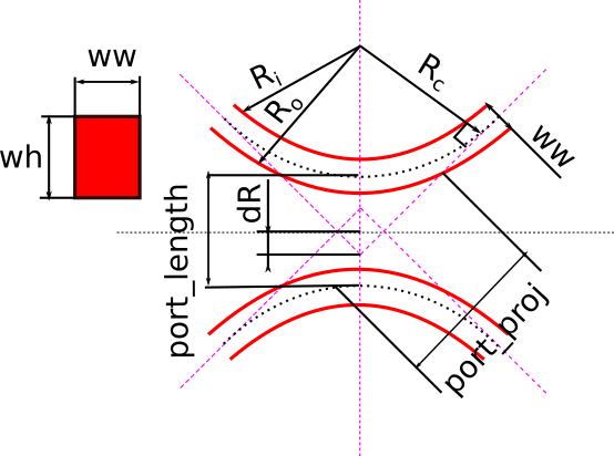
Here is the radius of the inner surface of the wire, is the radius of the outer surface of the wire. As you know, the angle between the radius of the circle and the tangent to the circle at this point is equal to , all angles in the models are equal to or .

I took the gap between the wires for powering equal to 1mm, from here:

Because of the need to have the feed gap, I slightly moved the "squares" apart, the measure of the "extension" is 2:

All arcs have length . The choice of a name for the variable is not really appropriate, but as it is :) Let's compose a system of equations describing the relationship between the elements of the structure:

The first equation of the system reflects the fact that the perimeter of one "square" should be related to the "quarters" of the wavelength. The second equation introduces the relationship between the lengths of the sides of the "square", it is not as obvious as the first equation, but it is derived quite simply.

I solve the system in Maxima:

(%i1) eq0:2*delta_port + quad_small + quad_big = 2*quad_size;
(%o1)         quad_small + quad_big + 2 delta_port = 2 quad_size
(%i2) eq1:quad_small = quad_big - dR*sqrt(2);
(%o2)                 quad_small = quad_big - sqrt(2) dR
(%i3) solve([eq0, eq1], [quad_small, quad_big]);
                     2 quad_size - 2 delta_port - sqrt(2) dR
(%o3) [[quad_small = ---------------------------------------,
                                        2
                         2 quad_size - 2 delta_port + sqrt(2) dR
              quad_big = ---------------------------------------]]
                                            2

The and unambiguously set the antenna model (as a function of wire parameters, radius of curvature and wavelength), now I can proceed to simulation.

Simulation

After I got my hands on modeling simple dipole antennas and a simple loop antennas, creating a model for Kharchenko's antenna was not too difficult (full text of the model). The mathematical model was described above, I chose the parameters based on common sense and materials available:

• , - my wire,
• Ohm - coaxial wire resistance,
• - I think this is a more or less normal rounding radius,
• - must be at least wavelength.

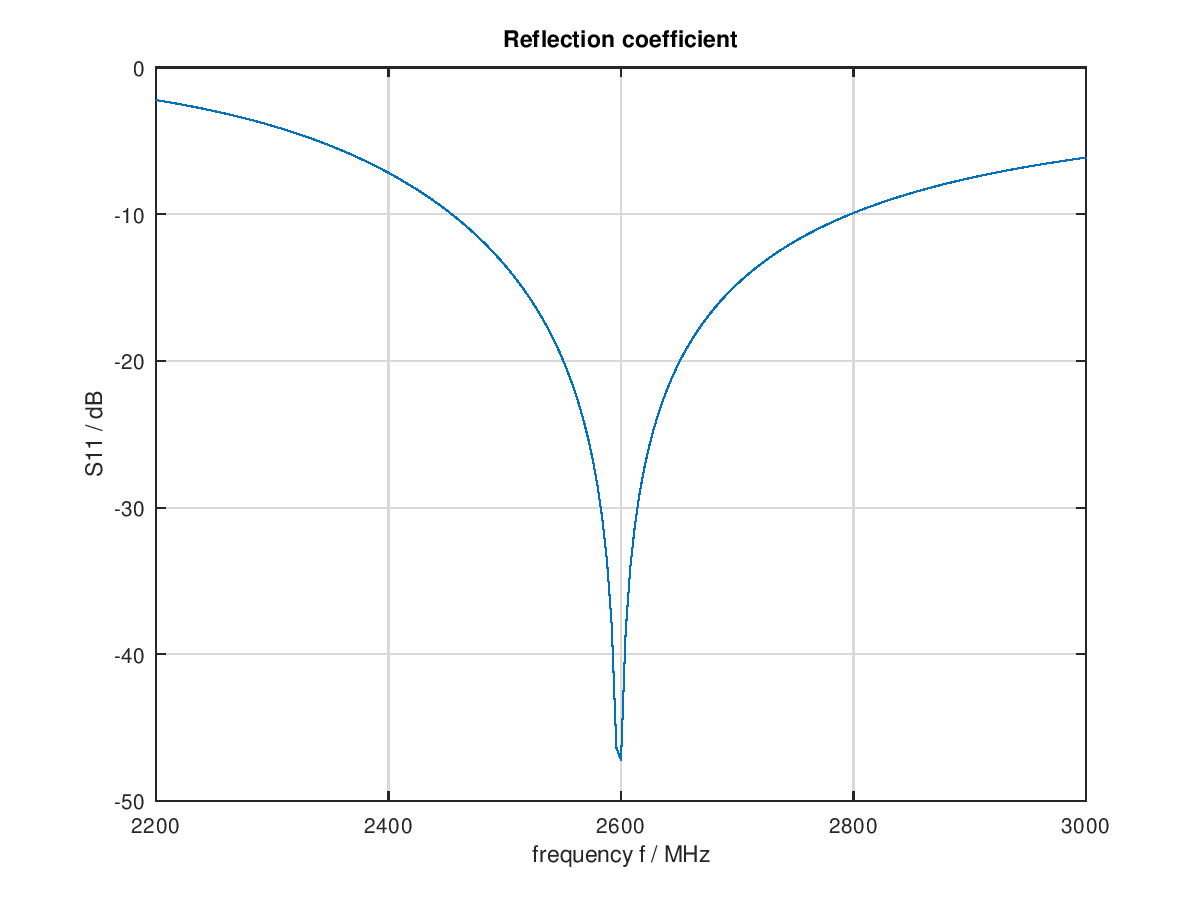
But the size of the side of the "square" I selected by running the simulation and achieving the minimum at my frequency of 2.6 GHz. And after that, I selected the distance from the middle of the wire to the reflector , achieving a resistance of 50Ohm (, ).

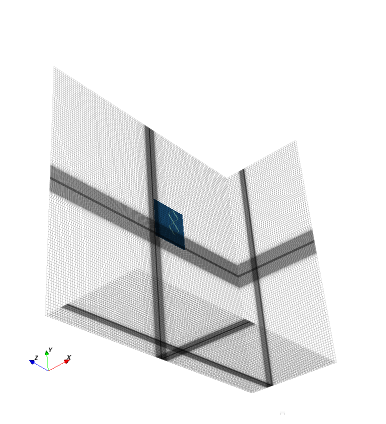
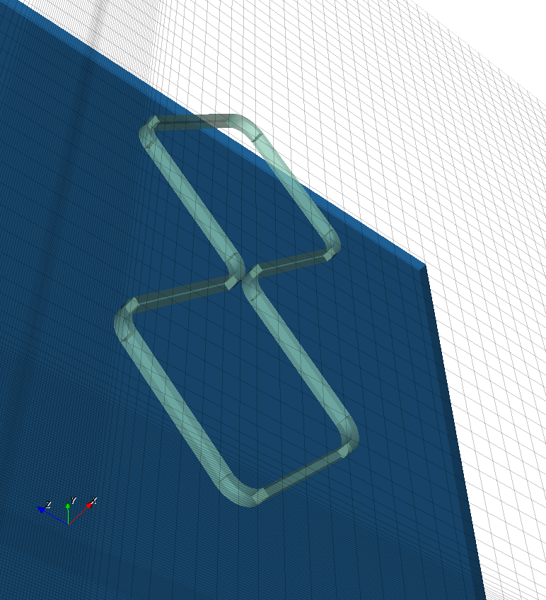
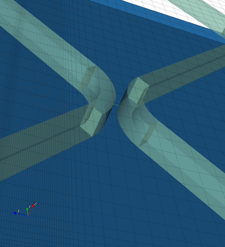
To reduce the calculation time while maintaining accuracy, I took advantage of the ability to specify an uneven mesh:

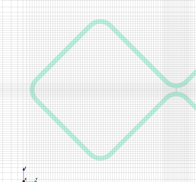
I tried to do so that as many surfaces as possible coincided with the grid lines: these are the wire planes along the axis, the reflector plane and the antenna feed gap.

Here are some more snapshots of the mesh and model:

1.

^ Antenna Theory and Design. Warren L. Stutzman, Gary A. Thiele

2.

^ These appear due to the aspect ratio in a right triangle with angles of : and

The actual simulation results:

Antenna directivity simulation video

directivity: Dmax = 10.6344 dBi I will count on this result.